- Binary classification;
- Linear Probability Model;
- Keeping probabilities between 0 and 1;
- Logistic function: a smoother model;
- Abandoning MSE because sensitive to outliers;
- Cross-entropy;
- Logistic Regression;
- Confusion Matrix (FP,TP,FN,TN);
- MCR;
- Precision/Recall.
The framework that we used to build a predictive model for regression followed four distinct steps:
- Decide on the mathematical form of the model: we used a linear model with potential for non-linear transformations and polynomials;
- Select a metric that defines the “best” fit: we used \(R^2\) or \(\mbox{(R)MSE}\);
- Estimate the coefficients of the model that are best using the training data: we found the coefficients that optimized our metric of choice on the training data;
- Evaluate predictive performance using test data: we calculated testing \(R^2\)/\(\mbox{(R)MSE}\) using a portion of the sample data that was withheld.
We used this process to build our first simple linear regression model to predict high school graduation rates but the same four steps are used by Zillow to build ZestimateTM, their deep learning model to predict house price.
These are also the same four steps that we will use as we shift in these notes to the task of classification. In a classification task, we try to predict a categorical target variable, very often a binary one (two-valued). Classification models are everywhere: they help doctors determine whether a patient has a disease, whether an image contains a particular object (say, a person or a cat), and whether a customer will purchase an item.
Example: Spam filters
Email spam, also referred to as junk email or simply spam, is unsolicited messages sent in bulk by email (spamming). The name comes from a Monty Python sketch in which the name of the canned pork product Spam is ubiquitous, unavoidable, and repetitive. A spam filter is a classification model that determines whether or not a message is spam based on properties of that message. Every mainstream email client, including Gmail, has a spam filter built in to ensure that the messages that get through to the user are genuine messages.
The Data
In order to build a spam filter, we’ll need a data set to train our model on. This data set must have as the unit of observation a single email message, record whether or not the message was spam (the target, \(Y\)), and record various variables of the message that are associated with being spam (the features, \(X_j\)). Such a data set, with nearly \(4000\) observations, can be found in the email data frame in the openintro library.
# A tibble: 3,921 × 21
   spam  to_multiple from     cc sent_email time                image attach
   <fct> <fct>       <fct> <int> <fct>      <dttm>              <dbl>  <dbl>
 1 0     0           1         0 0          2012-01-01 06:16:41     0      0
 2 0     0           1         0 0          2012-01-01 07:03:59     0      0
 3 0     0           1         0 0          2012-01-01 16:00:32     0      0
 4 0     0           1         0 0          2012-01-01 09:09:49     0      0
 5 0     0           1         0 0          2012-01-01 10:00:01     0      0
 6 0     0           1         0 0          2012-01-01 10:04:46     0      0
 7 0     1           1         0 1          2012-01-01 17:55:06     0      0
 8 0     1           1         1 1          2012-01-01 18:45:21     1      1
 9 0     0           1         0 0          2012-01-01 21:08:59     0      0
10 0     0           1         0 0          2012-01-01 18:12:00     0      0
# ℹ 3,911 more rows
# ℹ 13 more variables: dollar <dbl>, winner <fct>, inherit <dbl>, viagra <dbl>,
#   password <dbl>, num_char <dbl>, line_breaks <int>, format <fct>,
#   re_subj <fct>, exclaim_subj <dbl>, urgent_subj <fct>, exclaim_mess <dbl>,
#   number <fct>
We see in the leftmost column the target variable, spam, coded as \(0\) when a message is not spam and \(1\) when it is. The first feature, to_multiple, is a \(1\) if the message was sent to multiple people and \(0\) otherwise. cc records the number of people who are cc’ed on the email. winner (listed as a variable below the glimpse of the dataframe) records whether or not the word “winner” showed up in the message. You might be able to intuit the meaning of the remaining features by their names, but you can also read the help file, which describes each one.
These variables seem like they might be useful in predicting whether or not an email is spam, but take a moment to consider: how were we able to get our hands on data like this?
This particular data set arose from selecting a single email account, saving every single messages that comes in to that address over the course of a month, processing each message to create values for the predictor variables, then visually classifying whether or not the message is spam. That’s to say: this data represents a human’s best effort to classify spam and it cost a lot of resources. Can we build a model that will be able to identify the features that mark a message as spam so to automatically and classify future messages at a low cost?
Exploratory Data Analysis
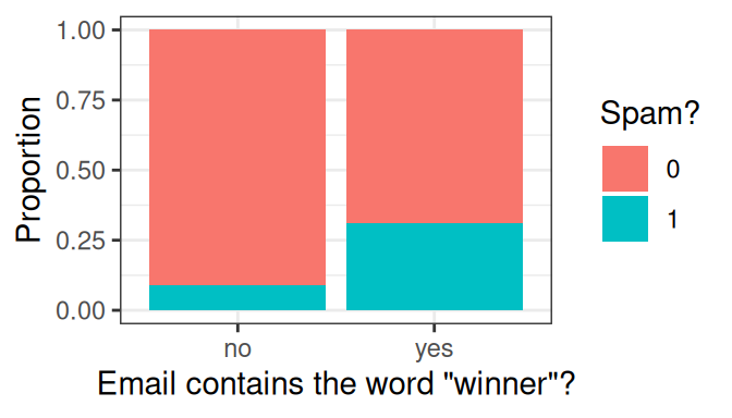
Let’s see how well a few tempting features work at separating spam from not spam by performing some exploratory data analysis. We might expect messages containing the word “winner” to be more likely to be spam than those that do not. A stacked, normalized bar chart can answer that question.
Indeed, it looks like around 30% of emails with “winner” were spam, compared to roughly 10% of those without. At this point, we could consider a very simple spam filter: if the message contains “winner”, then classify it as spam.
Although this is tempting, it is still a pretty weak classifier. Most of the messages with “winner” are not spam, so calling them spam will result in most of them being misclassified.
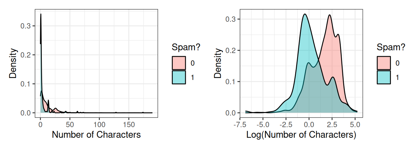
So if “winner” isn’t the silver bullet feature we need, let’s try another: num_char. This variable records the total number of characters present in the message (in thousands) – how long it is. We probably have no prior sense of whether spam would be more likely to consist of short or long emails, so let’s visualize them. This feature is numerical continuous, so let’s overlay two density plots to get a sense of the distribution between spam and not spam.
The original plot on the left is very difficult to read because this variable is heavily right-skewed: there are a small number of very long messages that obscure much of the data in the plot. On the right is a more useful visualization, one of the log-transformed version of the same variable.
We see a reasonable separation here: spam messages tend to be shorter than non-spam messages; so, we could consider a very simple spam filter: if the log number of characters is less than 1.2, classify it as spam.
However, this simple filter suffers from the same problem as the first. Although these density plots have the same area, there are in fact far fewer overall instances of spam than not-spam. That means that there are far more not-spam messages with a log number of characters less than 1.2 than there are spam message. This filter, like the first, would misclassify much of the training data.
What we need is a more general framework to fold the strength of these two variables - as well as many of the other ones in the data set - into a model that can produce a single, more accurate prediction. We will start from the framework of multiple linear regression and move to something that can be used for classification.
From Linear to Logistic Regression
Naive approach: Linear Probability Model
It would be nice if we could just retain all the awesome advantages of linear regression and carry them over to the problem of classification. We will see in a minute that we can keep only some some.
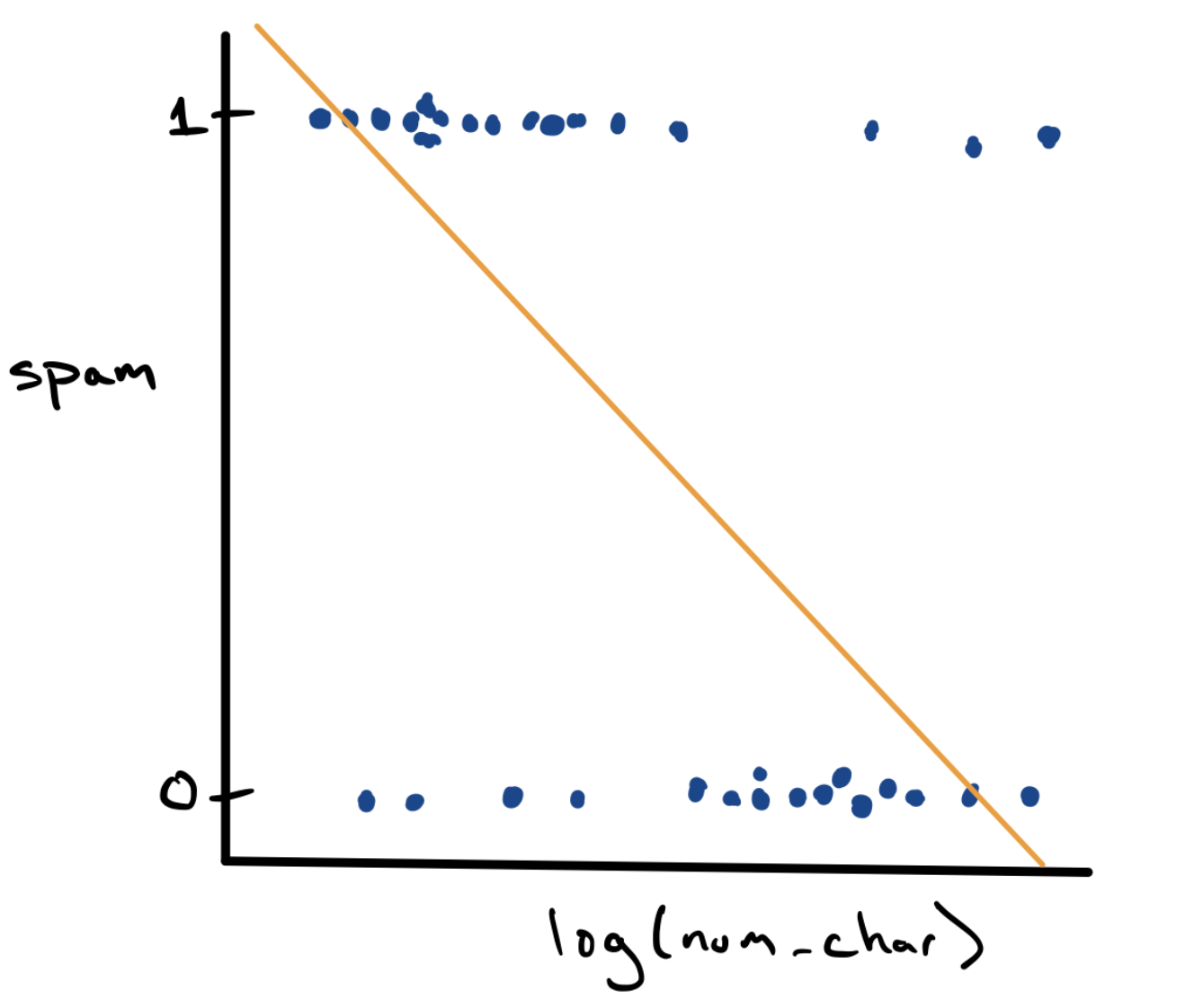
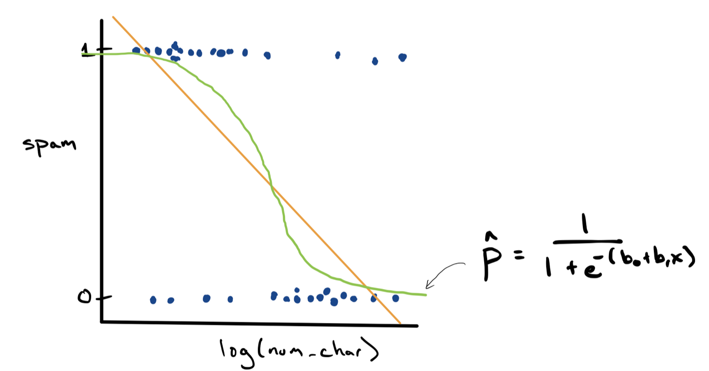
Let’s start by taking our existing simple linear regression model, applying it naively to this classification setting, and crossing our fingers. We can visualize the relationship between log_num_char and spam using an ordinary scatter plot.
This is a strange looking scatter plot - the dots can only take \(y\) values of 0 or 1 - but it does capture the overall trend observed in the density plots, that spam messages are longer. Since we have a scatter plot, we could fit a simple linear regression model using the method of least squares (in gold).
\[ \hat{Y} = b_0 + b_1 X \]
While this is doable, it leaves us with a few sppoky questions. The value of \(\hat{Y}\) can be anywhere on the real number line.
What does it mean if we predict that the value of \(Y=\) spam is .71? \(Y\) can only be 0 or 1 …
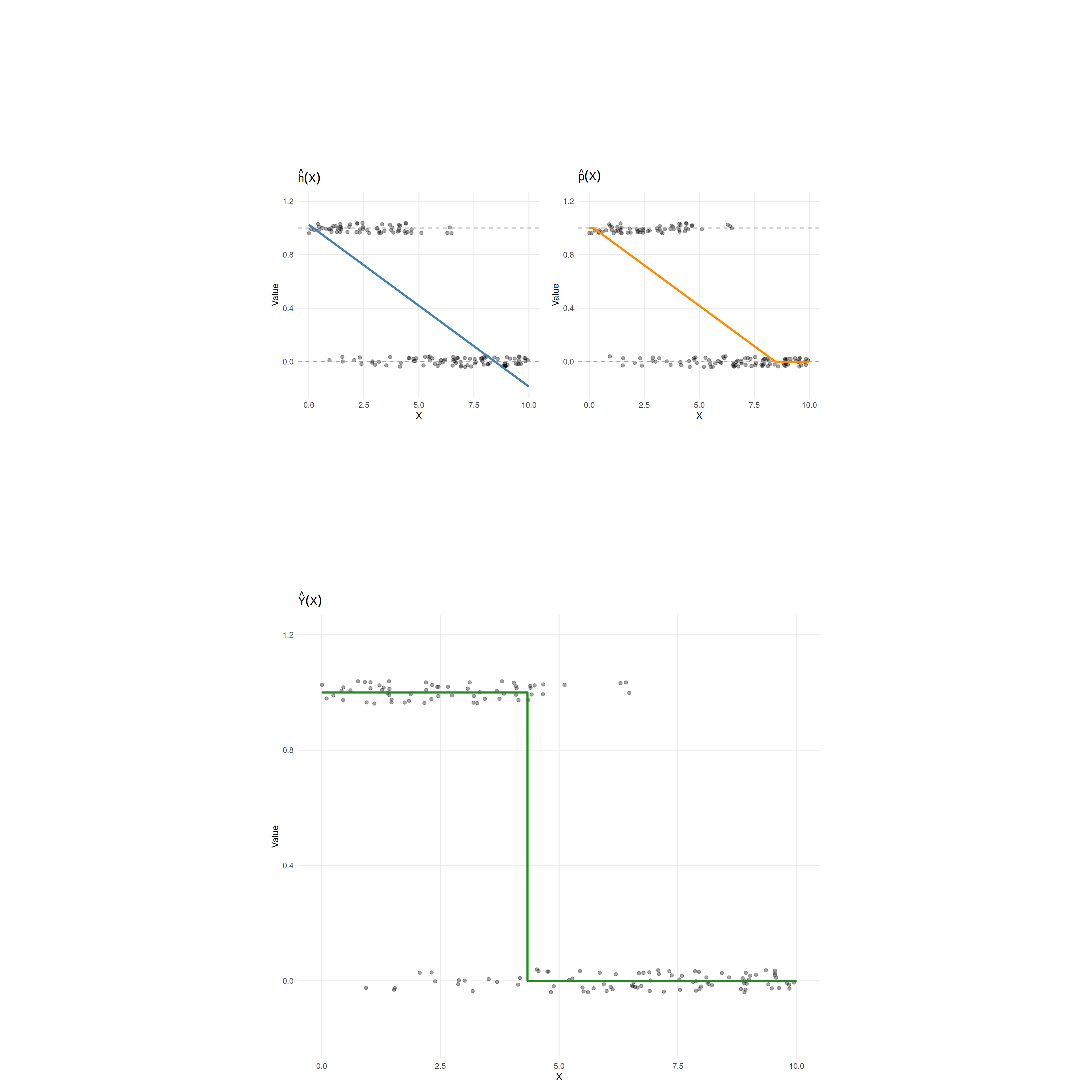
One approach to resolving this is to treat our equation not as a value of \(Y\), but as an estimate of the probability, \(p\), that \(Y = 1\) if I know the value of the feature X. We can rewrite the model as:
\[p(X) = b_0 + b_1 X\]
Then fit it
\[\hat{p}(X) = \hat{b}_0 + \hat{b}_1 X\]
Then we could predict \(Y=1\) by checking if this estimated probability is greater than \(0.5\), otherwise we predict 0. How does that sound?
\[
\hat{Y}(X) \equiv
\begin{cases}
0 & \text{if} \; \hat{p}(X) < 0.5 \\
1 & \text{if} \; \hat{p}(X) \geq 0.5
\end{cases}
\]
However… What if \(\hat{p}(\mathbf{X}) = 1.5\)? Or \(-30\)? Well, we can just cut off those values and make them equal to \(1\) or \(0\) respectively.
This is what we call a Linear Probability Model. If you must see a complete formal definition here it is:
def: Linear Probability Model (you don’t need to remember this)
If you have an \(n\)-sized sample of a binary target variable (\(Y_i = 0,1\)) and several features \(X_{1,i}, \ldots, X_{q,i}\).
Step 1 \[ h(\mathbf{X}) \equiv b_0 + b_1 X_1 + b_2 X_2 + \ldots + b_q X_q \]
which defines the helper function \(h()\) as the linear model.
Step 2
Fit it as usual, based on minimizing the MSE on the data, to obtain the OLS coefficients.
\[ \hat{b}_{0, OLS }, \hat{b}_{1, OLS }, \ldots, \hat{b}_{q, OLS } \]
and \[\hat{h}(\mathbf{X}) =\hat{b}_{0, OLS } + \hat{b}_{1, OLS } X_1, \ldots, \hat{b}_{q, OLS } X_q \].
Step 3
\[
\hat{p}(\mathbf{X}) \equiv \hat{P}(Y=1|\mathbf{X}) \equiv \begin{cases}
0 & \text{if} \; \hat{h} (\mathbf{X}) <0 \\
\hat{h} (\mathbf{X}) & \text{if} \; 0 \leq \hat{h} (\mathbf{X}) \leq 1 \\
1 & \text{if} \; \hat{h} (\mathbf{X}) > 0
\end{cases}
\]
which limits the actual estimated probability between 0 and 1.
Step 4 \[
\hat{Y} (\mathbf{X}) \equiv \begin{cases}
0 & \text{if} \; \hat{p} (\mathbf{X}) < 0.5 \\
1 & \text{if} \; \hat{p} (\mathbf{X}) \geq 0.5
\end{cases}
\]
which makes the final prediction about \(Y\).
where you have certainly recognized the estimated conditional probability \(\hat{P}(Y=1|\mathbf{X})\): the estimated probability that \(Y\) is equal to 1, knowing the value of the \(\mathbf{X}= X_1, X_2, \dots , X_q\).
The problem with this model is that it just behaves badly when we fit it on the data: it’s sensitive to outliers and has other unpleasant mathematical properties. Though the author of these notes finds it really pretty!
Getting gentler: the logistic model.
Ok, so, basically we have two problems
- we got a bit too … blunt(?) when clipping off the below 0 and above 1 values of the probability.
- optimizing \(\mbox{MSE}\) when fitting \(h(\mathbf{X})\) is just a bad idea, because it makes it sensitive to outliers
The Logistic function
Let’s start with the first problem.
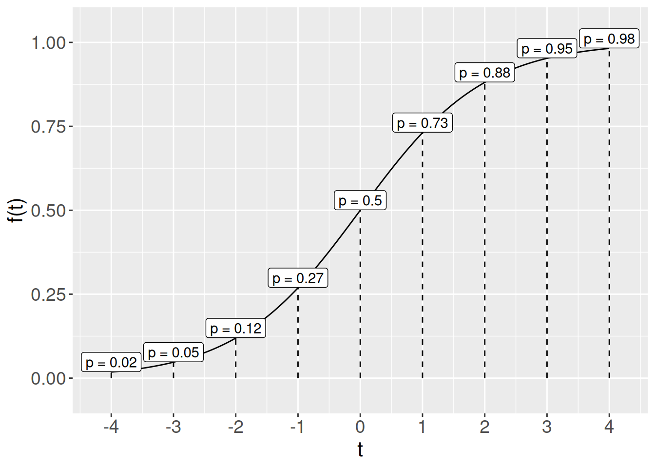
Instead of just setting \(p(\mathbf{X})\) abruptly to 0 and 1, we can use a smooth, gentle function that makes the probability limited between 0 and 1. Sucha function is called a sigmoid. The most commonly used sigmoid function is called the logistic function:
def: Logistic function
\[ f_{\sigma}(t) \equiv \frac{1}{1 + {\rm e}^{-t}}\]
We can fix this by changing the mathematical form of the model used to predict the response. Instead of it being a line, we can use an alternative function that prevents predictions greater than 1 and less than zero.
And here’s its graph.
\(t\) can be any number of the real number line. As \(t\) gets large, \(f_{\sigma}(t)\) approaches 1; as \(t\) is negative, \(f_{\sigma}(t)\) approaches 0; when \(t\) is 0, \(f_{\sigma}(t)\) is 0.5. Let’s build some intuition here:
| 0 |
\(\frac{1}{1 + e^{0}} = \frac{1}{1 + 1} = 1/2\) |
| -1 |
\(\frac{1}{1 + e^{1}} = \frac{1}{1 + e} = \frac{1}{1 + 2.72} \approx 0.27\) |
| 1 |
\(\frac{1}{1 + e^{-1}} = \frac{1}{1 + 1/e} = \frac{1}{1 + 0.368} \approx 0.73\) |
| -1,000,000 |
\(\frac{1}{1 + e^{1,000,000}} \approx \frac{1}{1 + \infty} \approx \frac{1}{\infty} \approx 0\) |
| 1,000,000 |
\(\frac{1}{1 + e^{-1,000,000}} = \frac{1}{1 + 1/e^{1,000,000}} \approx \frac{1}{1 + 0} \approx 1\) |
This is awesome because we can just stick the linear function \(h(\mathbf{X})\) inside of the sigmoid and obtain a number between 0 and 1, that we can interpret as a probability!
We could declare victory, go home, and have a feast, but… there’s bad news.
We still have the second problem.
Good-bye to Least Squares
Linearity is a beautiful thing. The Least-Squares algorithm is a way to optimize the MSE of your predictions when the predictions are in a linear form.
As I promised you, we will maintain some linearity but we can’t really keep pretending that MSE is a good way to measure the fitness of our predictions.
We will still have a function with a linear piece at its core:
\[
p(\mathbf{X})= \frac1{1 + {\rm e}^{-\left( b_0 + b_1 X_1 + b_2 X_2 + \ldots + b_q X_q \right)}}
\]
Look at it! How pretty! Tucked cozily up inside that exponent.
But the closeness of the estimation will be measured by a different function than the MSE. You don’t have to remember it. R will do the optimization for you, but I will include it here for completeness.
def: Sample Cross Entropy (you don’t need to remember this)
For a certain model estimating probability \(p(\mathbf{X})\) for binary data \(Y_i\), the cross entropy of the model measures how far the model estimate is from the data, and is defined mathematically by
\[ H \equiv -\frac1{n} \sum_{i=1}^n \left[ Y_i {\rm log} \left(p(\mathbf{X})\right) + \left(1-Y_i\right) {\rm log} \left(1-p(\mathbf{X})\right) \right] \]
This function is not as nice as the MSE, unfortunately. We can’t solve its minimization through calculus like the Ordinary Least Squares Method. We will be forced to use numerical methods to optimize it.
This feels like loss (let me know if you get the pun).
Putting it all together
def: Logistic Regression
If you have an \(n\)-sized sample of a binary target variable (\(Y_i = 0,1\)) and several features \(X_{1,i}, \ldots, X_{q,i}\).
Step 1 \[ P(Y=1|\mathbf{X}) = p(\mathbf{X})= \frac1{1 + {\rm e}^{-\left( b_0 + b_1 X_1 + b_2 X_2 + \ldots + b_q X_q \right)}} \]
which defines the logistic probability model as a function of the features. The \(b_0, b_1, \ldots, b_q\) are called the coefficients or weights of the model.
Step 2 \[
H (b_0, b_1, \ldots, b_q) \equiv -\frac1{n} \sum_{i=1}^n \left[ Y_i {\rm log} \left(p(\mathbf{X}_i)\right) + \left(1-Y_i\right) {\rm log} \left(1-p(\mathbf{X}_i)\right) \right]
\]
which defines the cross-entropy function for the logistic model. When the entropy is close to 0 the estimate of the probability is very good.
Step 3
Now we can use some numerical algorithm (like Gradient Descent or Nelder-Mead) to minimize \(H\) and find the optimal coefficients
\[
\hat{b}_{0, LR }, \hat{b}_{1, LR }, \ldots, \hat{b}_{q, LR }
\]
and then plug them in and get the estimated probability
\[
\hat{p}(\mathbf{X})= \frac1{1 + {\rm e}^{-\left( \hat{b}_{0,LR} + \hat{b}_{1,LR} X_1 + \hat{b}_{2,LR} X_2 + \ldots + \hat{b}_{q,LR} X_q \right)}}
\]
Step 4
\[
\hat{Y} (\mathbf{X}) \equiv \begin{cases}
0 & \text{if} \; \hat{p} (\mathbf{X}) < 0.5 \\
1 & \text{if} \; \hat{p} (\mathbf{X}) \geq 0.5
\end{cases}
\]
which makes the final prediction about \(Y\) just as we saw before.
We can visualize the approach that logistic regression takes by sketching the predictions as a green s-shaped curve on top of our scatter plot.
Evaluating our predictions (for classification)
Great, but how do we measure the goodness of our predictions \(\hat{Y}\)? I promise I’m not gonna blow your mind. This is going to be very unsurprising.
It’s in fact very similar to what we did with Hypothesis Testing (Remember Type I and Type II errors?)
Why? Because this is a discrete, binary variable! So it makes sense to compare the truth with your prediction and consider all the ways we could be correct or incorrect about it.
Hopefully, we will classify most of our e-mails correctly, but we will fail at least some of the time. We might predict that an e-mail is spam when it is not. In other cases, we might predict that an e-mail is not spam when it actually is. Therefore, there are two types of error we should consider.
Recall that based on the email dataset, 1 refers to an e-mail which is truly spam. In a binary classification problem, we often call a prediction of 1 a positive prediction. Likewise, a prediction of 0 is a negative prediction. This sets up formal definitions for the two types of errors mentioned above.
def: Confusion Matrix
Remember that \(Y\) means the true value of the target variable, and \(\hat{Y}\) is your prediction of it. Then we define
| \(\hat{Y} = 0\) |
true negatives (TN) |
false negatives (FN) |
| \(\hat{Y} = 1\) |
false positives (FP) |
true positives (TP) |
Out of these 4 sample quantities we can now build a series of different measures of performance of our model. Unfortunately there is no better or worse measure in absolute. Depending on your circumstances, you might care about one of these 4 numbers more than the others, etc…
def: Misclassification Rate (MCR)
This is an estimate of the probability of just being wrong (one way or the other)
\[\mbox{MCR} = \hat{P}(\hat{Y} \neq Y) = \frac{\mbox{FP} + \mbox{FN}}{n}\]
where \(n= \mbox{FP} + \mbox{TP} + \mbox{TN} + \mbox{FN}\) is the total sample size.
If you want to avoiding mixing together the two types of error you can instead use these two extremeley popular queantities: Precision and Recall.
def: Precision
This is an estimate of the probability that your positive predictions are correct
\[\mbox{Precision} = \hat{P}(Y=1 | \hat{Y} =1 ) = \frac{\mbox{TP}}{\mbox{TP} + \mbox{FP}}\]
I.e. the percentage of times you’re correct when you say “it’s spam!” is your Precision.
What’s the cheat to make your Precision = 1?
Just… never say something is spam…
Well technically then your precision is undefined but basically you’ll never make a false positive (FP = 0) if you never make a positive prediction, right?
But what’s the trade-off?
def: Recall
This is an estimate of the probability that the positive samples were correctly predicted by your model
\[\mbox{Recall} = \hat{P}(\hat{Y}=1 | Y =1 ) = \frac{\mbox{TP}}{\mbox{TP} + \mbox{FN}}\]
I.e. the percentage of times you say “it’s spam!” when a sample is actually spam is your Recall.
What’s the cheat to make your Recall = 1?
Just… say everything is spam…
You’ll never make a false negative (FN = 0) if you never make a negative prediction.
What’s the trade-off?
Because of these two cheats, we can never only use precision or only use Recall to evaluate a model but we have to use both at the same time, just like in th eGeneralization unit we used significance level and power together to evaluate our tests, and confidence level together with precision (interval width) to evaluate our confidence intervals.
Workflow and Overfitting
Nothing to see here. It’s all the same as before.
Just like in a linear Regression context, we can fit a suite of different models on the training set and evaluate their performance on the testing set. Now, our model type of choice is logistic regression and our evaluation metric is \(\mbox{MCR}\) or Precision and Recall, etc.
Overfitting works the same way. Evaluation will look awesome on the training sample but bad on the test sample.
Summary
Logistic Regression is a … classification algorithm (nothwithstanding the name) for a binary target variable. It makes a linear combination of the features using coefficients, like in linear regression, but then models the probability of the data being 1 (positive) by passing that combination through a sigmoid function (logistic function) that keeps it between 0 and 1. Then we optimize a new measure that replaces the MSE, called cross-entropy (H) through numerical methods, and find the optimal coefficients. Finally, if the estimated probability is larger than 0.5, we predict 1, otherwise 0.
We have also seen which measures of goodness can be used to evaluate classification algorithms: True/False Positives/Negatives, Misclassification Rate (MCR), Precision and Recall.