[1] 0 1 0 0 1 0 0 0 1 1[1] 0.4Discrete random variables, probability mass functions, cumulative distribution functions
In a previous tutorial, we saw that if we want to simulate tossing a fair coin \(10\) times, and compute the proportion of times that the coin lands heads, we could use the function sample() to sample from (0, 1), where the outcome “Heads” is represented by the number 1 and the outcome “Tails” is represented by the number 0. Our code might look like:
set.seed(1)
tosses_10 <- sample(c(0,1), 10, replace = TRUE)
tosses_10
mean(tosses_10)
[1] 0 1 0 0 1 0 0 0 1 1[1] 0.4We used the same idea, of assigning numbers to outcomes when we looked at the probability distribution of the number of heads in three tosses, and when we defined the Bernoulli, binomial, and hypergeometric distributions. Once we assign numbers to non-numeric outcomes, we can then do mathematical operations on these numbers, for example, we could analyze them, compute proportions, and so on, that we could not do otherwise.
We will need this incredibly important and useful notion of representing abstract or non-numeric outcomes and data as numbers - we call them Random Variables: “random” because the numbers have associated probabilities (because the outcomes they represent have probabilities), and “variables” because they take different values.
Random variables simplify notation, and allow us to analyze all types of data. They are absolutely central to statistics, and as budding statisticians, eager to get on to the good stuff like statistical inference, you need to understand what they are and how to use them.
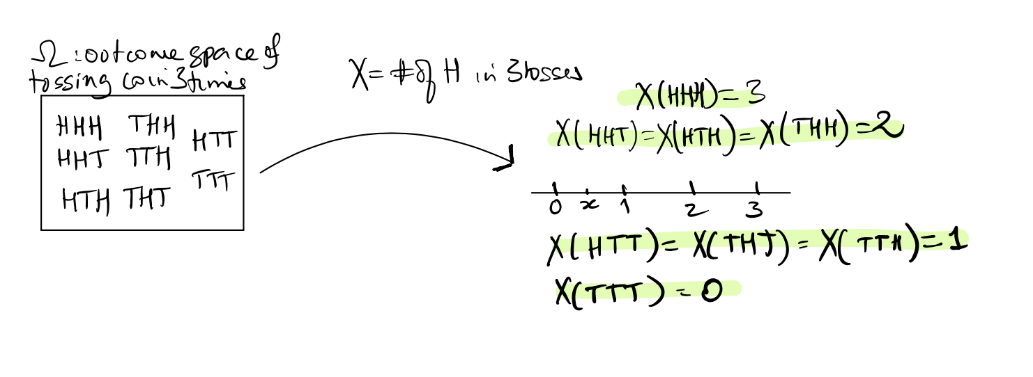
When we tossed a coin three times and counted the number of heads, we defined an outcome space \(\Omega\), and then defined a function that mapped the each of the outcomes in the set \(\Omega\) to a real number. That is, we know that \(\Omega\) is the set \(\{HHH, TTT, HHT, HTH, THH, TTH, THT, HTT\}\), we mapped the outcome \(HHH\) to the real number \(3\), the outcome \(TTT\) to the real number \(0\), each of the outcomes \(HHT, HTH, THH\) to the number \(2\), and each of the outcomes \(TTH, THT, HTT\) to the number \(1\). So each of the 8 outcomes is assigned to either \(0, 1, 2\), or \(3\). In this way, we used numbers instead of sequences of heads and tails.
In the simulation above, sampling over and over again from (0,1), we got a sequence of \(0\)’s and \(1\)’s that was randomly generated by our sampling. Once we had numbers (instead of sequences of heads and tails), we were able to do operations using these numbers, such as compute the proportion of times we sampled \(1\), or represent the probabilities as a histogram. Moving from non-numeric outcomes in an outcome space \(\Omega\) to numbers on the real line is enormously useful.
In mathematical notation:
\[ X : \Omega \rightarrow \mathbb{R}\]
\(X\) is called a random variable.
For example, suppose we draw two penguins from our penguin data set (so we pick two rows from the data frame), and count the number of Gentoo penguins in our sample, calling this number \(X\). Then \(X\) could be 0, 1, or 2, depending on how many Gentoo penguins we draw. If we draw without replacement, what is the probability that \(X = 2\)?
Note that for \(X = 2\), both draws have to be Gentoo, so the first draw has to be a Gentoo penguin, as well as the second. There are 344 penguins, of which 124 are Gentoo.
The probability that the first penguin drawn is Gentoo is \(\dfrac{124}{344}\) and the probability that the second is Gentoo given that the first is Gentoo is a conditional probability.
We can compute this probability using the definition of conditional probability:
\(P\)(2nd penguin Gentoo | first is Gentoo) \(= \dfrac{123}{343}\).
So the probability that both penguins are Gentoo is, using the multiplication rule, \[ \dfrac{124}{344} \times \dfrac{123}{343}\approx 13\% \] (The wiggly equal to sign (\(\approx\)) means “approximately equal to”.)
\(\{X = x\}\) is an event in \(\Omega\) consisting of all the outcomes that are mapped to the number \(x\) on the real line. The probability of such events is written as \(P(X = x)\). For example, if we roll a pair of dice, and let \(X\) denote the sum of the spots, then the event \(\{X = 4\}\) consists of the outcomes {(,), (,), (, )}.
What we are doing is creating a mathematical notation that formalizes the association of outcomes in \(\Omega\) with numbers. We have associated outcomes with numbers before, in the previous chapters discussing probability, and in the worksheets. We are just explicitly defining what we did.
Earlier we defined probability distributions as describing how the total probability of \(1\) or \(100\)% was distributed among all possible outcomes in \(\Omega\). Now we can extend this definition to the associated real numbers using \(X\), and so we get a probability distribution on the range of \(X\).
For example, consider the familiar example of the outcome space of three tosses of a fair coin. We can define the random variable \(X\) to be the number of heads, and represent it as in the picture below:
Just as with data types, random variables can be classified as discrete or continuous:
Continuous random variables can take any value in some specified interval, where the interval might be the entire real line.
In all of the following, we do not restrict the values taken by the random variable, and the values can be anything in some interval.

Recall that American roulette wheels have 38 numbered slots: 36 are numbered 1 through 36 (18 red and 18 black) and two green slots are numbered 0 and 00. As the wheel spins, a ball is sent spinning in the opposite direction. When the wheel slows the ball will land in one of the numbered slots.
Players can make various bets on where the ball lands, such as betting on whether the ball will land in a red slot or a black slot. If a player bets one dollar on red, and the ball lands on red, then they win a dollar, in addition to getting their stake of one dollar back, so they gain one dollar.
If the ball does not land on red, then they lose their dollar to the casino. Suppose a player bets one dollar on red on each of six consecutive spins. Their net gain can be defined as the amount they won minus the amount they lost. Is net gain a random variable? What are its possible values (think about their net gain if they win all 6 times, or win 5 times and lose once etc.)?
Yes, net gain is a random variable, because its value is a number determined by the outcome of a random experiment (the six spins of the wheel). The possible values of net gain are: \(-6, -4, -2, 0, 2, 4, 6\).
Why is this? Why are they all even? Trading one loss for one win raises net gain by \(2\) dollars: they avoid losing \(1\) dollar and gain \(1\) dollar instead. If they win \(W\) times, they lose \(6 - W\) times, so net gain is \(W - (6 - W) = 2W - 6\). The possible values of \(W\) are \(0, 1, 2, \ldots, 6\) (\(W=0\) corresponds to winning none of the spins, \(W=6\) corresponds to winning all of them), and the associated values of net gain \(=2W - 6\) are given by \(-6, -4, \ldots, 6\), as summarized in the table below:
| Wins | 0 | 1 | 2 | 3 | 4 | 5 | 6 |
|---|---|---|---|---|---|---|---|
| Losses | 6 | 5 | 4 | 3 | 2 | 1 | 0 |
| Net gain | −6 | −4 | −2 | 0 | 2 | 4 | 6 |
Recall that the probability distribution of \(X\) lists each possible value of \(X\) with its probability. We can list the values and corresponding probability in a table. This table is called the distribution table of the random variable. For example, let \(X\) be the number of heads in \(3\) tosses of a fair coin. The probability distribution table for \(X\) is shown below. The first column should have the possible values that \(X\) can take, denoted by \(x\), and the second column should have \(P(X = x)\). Make sure that the probabilities add up to 1! \(\displaystyle \sum_x P(X = x) = 1\).
| \(x\) | \(P(X = x)\) |
|---|---|
| \(0\) | \(\displaystyle \frac{1}{8}\) |
| \(1\) | \(\displaystyle \frac{3}{8}\) |
| \(2\) | \(\displaystyle \frac{3}{8}\) |
| \(3\) | \(\displaystyle \frac{1}{8}\) |
We can write down the definition of the function \(f(x)\) and it gives the same information as in the table:
\[ f(x) = \begin{cases} \frac{1}{8}, \; x = 0, 3 \\ \frac{3}{8}, \; x = 1, 2 \\ 0, \; \text{otherwise} \end{cases} \]
We see here that \(f(x) > 0\) for only \(4\) real numbers, and is \(0\) otherwise. We can think of the total probability mass as \(1\), and \(f(x)\) describes how this mass of \(1\) is distributed among the real numbers. It is often easier and more compact to define the probability distribution of \(X\) using \(f\) rather than the table.
Let’s revisit the special distributions that we have seen so far.
For each of the named distributions that we defined earlier, we can define a random variable with that probability distribution.
Let \(X\) take the values \(1, 2, 3, \ldots, n\) with \(P(X = k) = \displaystyle \frac{1}{n}\) for each \(k\) from \(1\) to \(n\). We call \(X\) a discrete uniform random variable with \(P(X = k) = \displaystyle \frac{1}{n}\) for \(1 \le k \le n\). Recall that \(n\) is the parameter of the discrete uniform distribution, and we write \(X \sim\) Discrete Uniform\((n)\).
Suppose we roll a pair of dice and sum the spots, and let \(X\) be the sum. Is \(X\) a discrete uniform random variable?
No. \(X\) takes discrete values: \(2, 3, 4, \ldots, 12\), but we knokw that these are not equally likely. Recall that, for example, \(P(X = 2) = \dfrac{1}{36}\) but \(P(X = 7) = \dfrac{6}{36}\)
Recall that the Bernoulli distribution describes the probabilities associated with random binary outcomes that we designate as success and failure, where \(p\) is the probability of a success. We can define \(X\) to be a random variable that takes the value \(1\) with probability \(p\), and the value \(0\) with probability \(1-p\). \(X\) is called a Bernoulli random variable, and it indicates whether the outcome of the random experiment or trial was a success or not. We say that \(X\) is Bernoulli with parameter \(p\), and write \(X \sim\) Bernoulli\((p)\). Below are the same probability histograms that we have seen in the last chapter, but now they describe the probability mass function of \(X\).

Recall that the binomial distribution describes the probabilities of the total number of successes in \(n\) independent Bernoulli trials. We let \(X\) be this total number of successes (think tossing a coin \(n\) times, and counting the number of heads). Then we say that \(X\) has the binomial distribution with parameters \(n\) and \(p\), and write \(X \sim Bin(n,p)\), where \(X\) takes values in \(\{0, 1, 2, \ldots, n\}\), and \[P(X = k ) = \binom{n}{k} p^k (1-p)^{n-k}. \] Recall that the binomial coefficient 1 \(\displaystyle \binom{n}{k} = \frac{n!}{k!(n-k)!}.\)
In 2024, California elected Adam Schiff to the United States Senate by a wide margin over Republican candidate Steve Garvey. Schiff had a more difficult race in the primaries. The top four candidates in the California Senate race had their final debate on February 20, 2024, before the primary elections were held in March. In the California Elections and Policy Poll, conducted on January 21-29, 2024 2, Adam Schiff was the favorite candidate in the California Senate primary election, preferred by \(25\%\) of likely voters (he eventually received \(31.6\%\) of the votes). The primary elections in California decide the top two candidates (regardless of political affiliation) who will compete in the general election.
Suppose we had surveyed \(10\) likely voters in California, sampling them with replacement from a database of voters, what is the probability that more than \(2\) of the individuals in our sample would have preferred Adam Schiff over the other candidates for CA Senator?
In this example, since we are counting the number of voters in our sample that prefer Adam Schiff, such a voter would count as a “success”, because a success is whatever outcome we are counting (regardless of whom we may prefer). We can now set up our random variable \(X\):
Let \(X\) be the number of voters in our sample of ten voters who like Adam Schiff best among all the Senatorial candidates in California.
Then \(X \sim Bin(10, p = 0.25)\). (Why are these the parameters?) Using the complement rule, and the addition rule (for mutually exclusive events), we get:
\(P(X > 2) = 1 - P(X \le 2) = 1 - \left(P(X = 0) + P(X = 1) + P(X = 2)\right)\).
This gives us:
\[ \begin{aligned} P(X > 2) &= 1 - \left(\binom{10}{0}(0.25)^0 (0.75)^{10} + \binom{10}{1}(0.25)^1 (0.75)^9 + \binom{10}{2}(0.25)^2 (0.75)^8 \right)\\ & \approx 0.474\\ \end{aligned} \]
As stated earlier, we can define events by the values taken by random variables. For example, let \(X \sim Bin(10,0.4)\). In words \(X\) counts the number of successes in 10 trials. Given this \(X\), what are the following events in words?
\(X\) is the number of successes in ten trials, where the probability of success in each trial is 40%. \(X = 5\) is the event that we see exactly five successes in the ten trials, while \(X \le 5\) is the event of seeing at most five successes in ten trials. The last event, \(3 \le X \le 8\) is the event of at least three successes, but not more than eight, in ten trials.
In the example above, we sampled \(10\) California residents with replacement from a database of voters. Usually we sample without replacement, so if \(X\) is the number of successes in a simple random sample of \(n\) draws from a population of size \(N\), then \(X\) will have the hypergeometric distribution with parameters \(\left(N, G, n\right)\) where \(G\) is the total number of successes in our population.
We write this as \(X \sim HG(N, G, n)\). Recall that the probabilities of \(X\) are given by: \[ P(X = k) = \frac{\binom{G}{k} \times \binom{N-G}{n-k}}{\binom{N}{n}} \] where \(N\) is the size of the population, \(G\) is the total number of successes in the population, and \(n\) is the sample size. We denote the number of success in the sample by \(k\). It can take the values \(0, 1, \ldots, n\) or \(0, 1, \ldots, G\), if the number of successes in the population is smaller than the sample size, as long as we have enough failures in the population for \(k\) to be \(0\).
Of course, if the sample size \(n\) is more than the total number of failures in the population, then \(k\) has to be bigger than \(0\). For example, \(N=20, G = 12, n = 10\). There are only \(8\) non-successes, so at least \(2\) of the \(10\) draws must be successes.)
A supermarket chain in Florida (with about 1,000 employees eligible for training) occasionally selects employees to receive management training. A group of women there claimed that female employees were passed over for this training in favor of their male colleagues. The company denied this claim. (A similar complaint of gender bias was made about promotions and pay for the 1.6 million women who work or who have worked for Wal-Mart. The Supreme Court heard the case in 2011 and ruled that the case could not proceed as a class action.)3 If we set this up as a probability problem, we might ask the question of how many women have been selected for management training in the last 10 years. In order to do the math, we can simplify the problem. Suppose no women had ever been selected in 10 years of annually selecting one employee for training. Further, suppose that the number of men and women were equal, and suppose the company claims that it draws employees at random for the training, from the 1,000 eligible employees. If \(X\) is the number of women that have been picked for training in the past 10 years, what is \(P(X = 0)\)?
Note that we are picking a sample of size 10 without replacement and counting the number of women in our sample and therefore, a “success” will be selecting a woman. Modeling \(X\) as a hypergeometric random variable, we have that \(N = 1000\), there are 1,000 employees, and since half are women, we have \(G = 500\) women and \(N - G = 500\) men.
We want to compute the probability that out of the \(10\) employees that were selected at random from the \(1,000\) employees, none are women. This gives us, using the formula above:
\[P(X = 0) = \frac{\binom{500}{0} \times \binom{500}{10}}{\binom{1000}{10}}\approx 0.00093\] We will see later how to compute this probability in R.
There are three very important distributions that we see over and over again in many situations. One of them is the binomial distribution, which we have discussed above. The reason this distribution is so ubiquitous is that we use it for classifying things into binary outcomes and counting the number of “successes”. The second important discrete distribution is used to model many different things: from the number of people arriving at an ATM in a given period of time, to the frequency with which soldiers in the Prussian army were accidentally kicked to death by their horses4. This distribution is called the Poisson distribution after a French mathematician, Siméon-Denis Poisson, who developed the theory in the nineteenth century. Interestingly, he was not the first French mathematician to develop this theory. That honor belonged to the mathematician who was a contemporary (and friend) of Isaac Newton, Abraham de Moivre.5 (The third important distribution is called the Normal distribution, also first discovered by de Moivre, which we will introduce later in the course.)
The Poisson distribution appears in situations when we have a very large number of trials in which we are checking the occurrence or not of a particular event which has a very low probability. That is, we have a very large number \(n\) of Bernoulli trials, which have a very small \(p\) or probability of success, such that the product \(np\) is not too small or large. We call the number of successes \(X\), and it counts the occurrence of events whose counts tend to be small. Note that \(X \sim Bin(n, p)\), and \[P(X = 0) = \binom{n}{0}\times p^0\times (1-p)^n = (1-p)^n.\] For large \(n\), it turns out that \((1-p)^n \approx e^{-\lambda}\), where \(\lambda = np\). (Recall from calculus the constant \(e, \approx 2.71828,\) that is the base for the natural log and the exponential functions.). We won’t derive the distribution here, but we will use the Poisson distribution for random variables that count the number of occurrences of events in a given period of time in when the events result from a very large number of independent trials. The independence of the trials means one trial does not affect another. We also assume that the probability of success does not change over time.
This example was made famous by Ladislaus Bortkiewicz in 1898 when he discussed how a Poisson distribution fit the data he obtained from 14 corps in the Prussian cavalry over a period of 20 years.
Note that death by horse-kicks was quite rare with less than 1 death per corps per year (0.7 deaths per corps per year), over the 280 observations. Bortkiewicz recorded the number of deaths per corps per year, and just over half of the 280 observations (14 corps recorded over 20 years) had no deaths.
Let’s look at the empirical histogram of the data.

This is the shape we expect when we look at the distribution of a Poisson random variable, where a very low number of events has a much higher probability than larger numbers, so we have a right-skewed distribution.
Both the binomial and the hypergeometric distributions deal with counting the number of successes in a fixed number of trials with binary outcomes. The difference is that for a binomial random variable, the probability of a success stays the same for each trial, and for a hypergeometric random variable, the trials are not independent. The probability of a success on a trial depends on what was drawn before. If we use a box of tickets to describe these random variables, both distributions can be modeled by sampling from boxes with each ticket marked with \(0\) or \(1\), but for the binomial distribution, we sample \(n\) times with replacement and count the number of successes by summing the draws; and for the hypergeometric distribution, we sample \(n\) times without replacement, and count the number of successes by summing the draws.
Note that when the sample size is small relative to the population size, there is not much difference between the probabilities if we use a binomial distribution vs using a hypergeometric distribution. Let’s look at the gender discrimination example again, and pretend that we are sampling with replacement. Now we can use the binomial distribution to compute the chance of never picking a woman. Let \(X\) be defined as before, as the number of women selected in \(10\) trials.
\[ P(X = 0) = \binom{10}{0}\times\left(\frac{1}{2}\right)^0\times\left(\frac{1}{2}\right)^{10} = 0.0009765625 \approx 0.00098 \]
Recall that the probability using the hypergeometric distribution was 0.0009331878. You can see that the values are very close to each other. This is an illustration of the fact that we can use a binomial random variable to approximate a hypergeometric random variable if the sample size \(n\) is very small compared to the population size \(N\).
Now we will define another important quantity related to random variables. This quantity, called the cumulative distribution function, is another way to describe the probability distribution of the random variable.
The cdf is a very important function since it also describes the probability distribution of \(X\). In order to compute \(F(x)\) for any real number \(x\), we just add up all the probability so far: \[ F(x) = \sum_{y \le x} f(y) \]
For example, if \(X\) is the number of heads in \(3\) tosses of a fair coin, recall that:
\[ f(x) = \begin{cases} \displaystyle \frac{1}{8}, \; x = 0, 3 \\ \displaystyle \frac{3}{8}, \; x = 1, 2 \\ 0, \; \text{otherwise} \end{cases} \]
In this case, \(F(x) = P(X\le x) = 0\) for all \(x < 0\) since the first positive probability is at \(0\). Then, \(F(0) = P(X \le 0) = 1/8\) after which it stays at \(1/8\) until \(x = 1\). Look at the graph below:

Notice that \(F(x)\) is a step function, and right continuous. The jumps are at exactly the values for which \(f(x) > 0\). We can get \(F(x)\) from \(f(x)\) by adding the values of \(f\) up to and including \(x\), and we can get \(f(x)\) from \(F(x)\) by looking at the size of the jumps.
Suppose $X $ Bernoulli\((0.5)\). Then we know that \(P(X = 0) = P(X=1) = 0.5\). The cdf of \(X\), \(F(x)\) gives us the total probability so far up to and including \(x\). For example, if \(x = -3\), \(F(x) =0\) since the first time there is any positive probability for \(X\) is at \(0\). At \(x = 0\), \(F(x) = 0.5\), and it stays there until it gets to \(x =1\), when it “accumulates” another \(0.5\) of probability. Here is the figure:
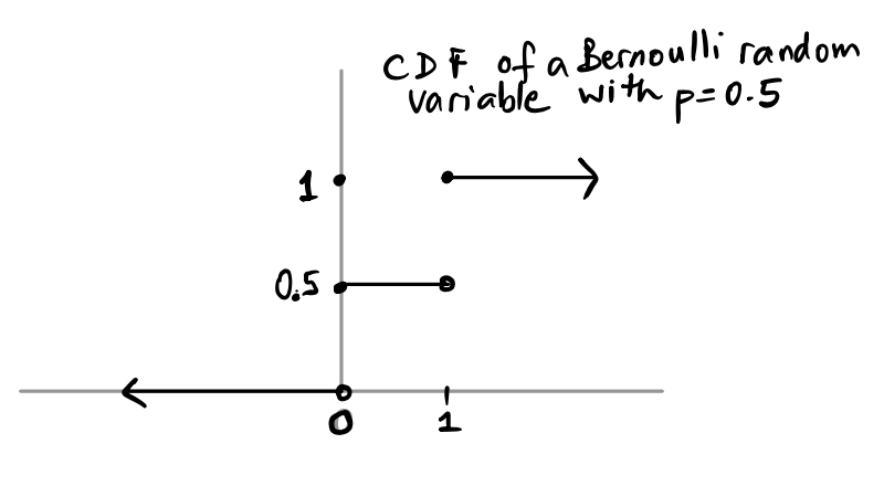
Notice where the function is open and closed (\(\circ\) vs \(\bullet\)).
Let \(X\) be the random variable defined by the distribution table below. Find the cdf of \(X\), and draw the graph, making sure to define \(F(x)\) for all real numbers \(x\). Before you do that, you will have to determine the value of \(f(x)\) for \(x = 4\).
| \(x\) | \(P(X = x)\) |
|---|---|
| \(-1\) | \(0.2\) |
| \(1\) | \(0.3\) |
| \(2\) | \(0.4\) |
| \(4\) | ?? |
Since \(\displaystyle \sum_x P(X = x) = \sum_x f(x) = 1\), \(f(4) = 1-(0.2+0.3+0.4) = 0.1.\) Therefore \(F(x)\) is as shown below.

sample()).