format_data <- data.frame(name = c("Evelyn", "Grace", "Juan", "Alex", "Monica", "Sriya"),
                 group = c("pdf", "pdf", "pdf", "website", "website", "website"),
                 understanding = c("deep", "shallow", "deep", "deep", "shallow",
                                   "shallow"),
                 major = c('Statistics', 'Economics', 'Economics', 'Statistics',
                           'Economics', 'Statistics'),
                 GPA = c(3.81, 3.63, 3.20, 2.85, 3.19, 3.80),
native_speaker = c('Yes','No','Yes','No','Yes','Yes'))Randomized Experiments
Principles of experimental design
Ideas in Code
First we create a data frame to store the pdf vs. website data.
The cobalt package in R contains the function bal.tab to create tables of standardized differences. By passing its output to plot you can create a Love plot. Note that cobalt expect treatment variables to be numeric or logical, so we begin by converting group to the logical variable is_website.
library(cobalt)
format_data <- format_data |>
                mutate(is_website = group == 'website')

bal.tab(is_website ~ major + GPA + native_speaker, data = format_data,
        s.d.denom = 'pooled', binary = 'std') |>
  plot()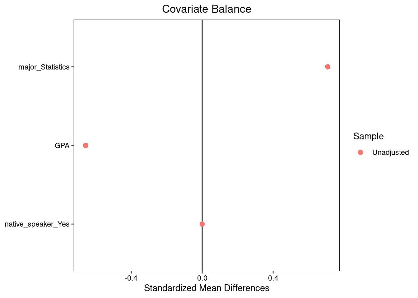
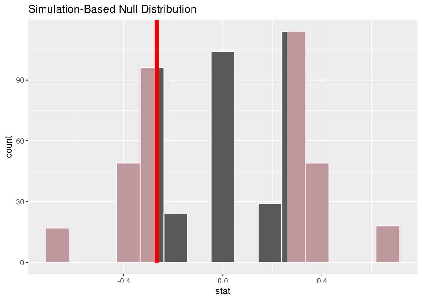
Running balance tests uses infer much like we did in the generalization unit. The covariate for which we are testing balance is the response and the treatment is the explanatory variable.
library(infer)
set.seed(2024-3-25)
obs_stat <- format_data |>
   specify(explanatory = group,
          response = GPA) |>
  calculate(stat = "diff in means", order = c("website","pdf"))

null <- format_data |>
  specify(response = GPA,
          explanatory = group) |>
  hypothesize(null = "independence") |>
  generate(reps = 500, type = "permute") |>
  calculate(stat = "diff in means", order = c("website","pdf"))

null |>
  visualize() +
  shade_p_value(obs_stat, direction = 'both')