The Taxonomy of Data

Vectors and Data Frames

The concepts of a variable, its type, and the structure of a data frame are useful because they help guide our thinking about the nature of a data. But we need more than definitions. If our goal is to construct a claim with data, we need a tool to aid in the construction. Our tool must be able to do two things: it must be able to store the data and it must be able to perform computations on the data. This is where R comes in!

First, we will discuss how R can store and perform computations on data. Then, we will relate these basics to the Taxonomy of Data we have just discussed.

R and RStudio

R is one of the most powerful languages for doing statistics and data science. One of the reasons for its power and popularity is that it is both free and open-source. This turns languages like R into something that resembles Wikipedia: a collaborative effort that is constantly evolving. Extensions to the R language have been authored by professional programmers¹, people working in industry and government², professors³, and students like you⁴.

You’ll be writing and running code through an app called RStudio. Beyond writing R code, RStudio allows you to manage your files and author polished documents that weave together code and text. RStudio can be run through a browser and we have set up an account for you that you can access by sending a browser tab to https://stat20.datahub.berkeley.edu/ or clicking the link in the upper right corner of the course website.

When you log into RStudio, the place where you can type and run R code is called the console and it’s located right here:

Figure 1: The R console in RStudio.

Code along

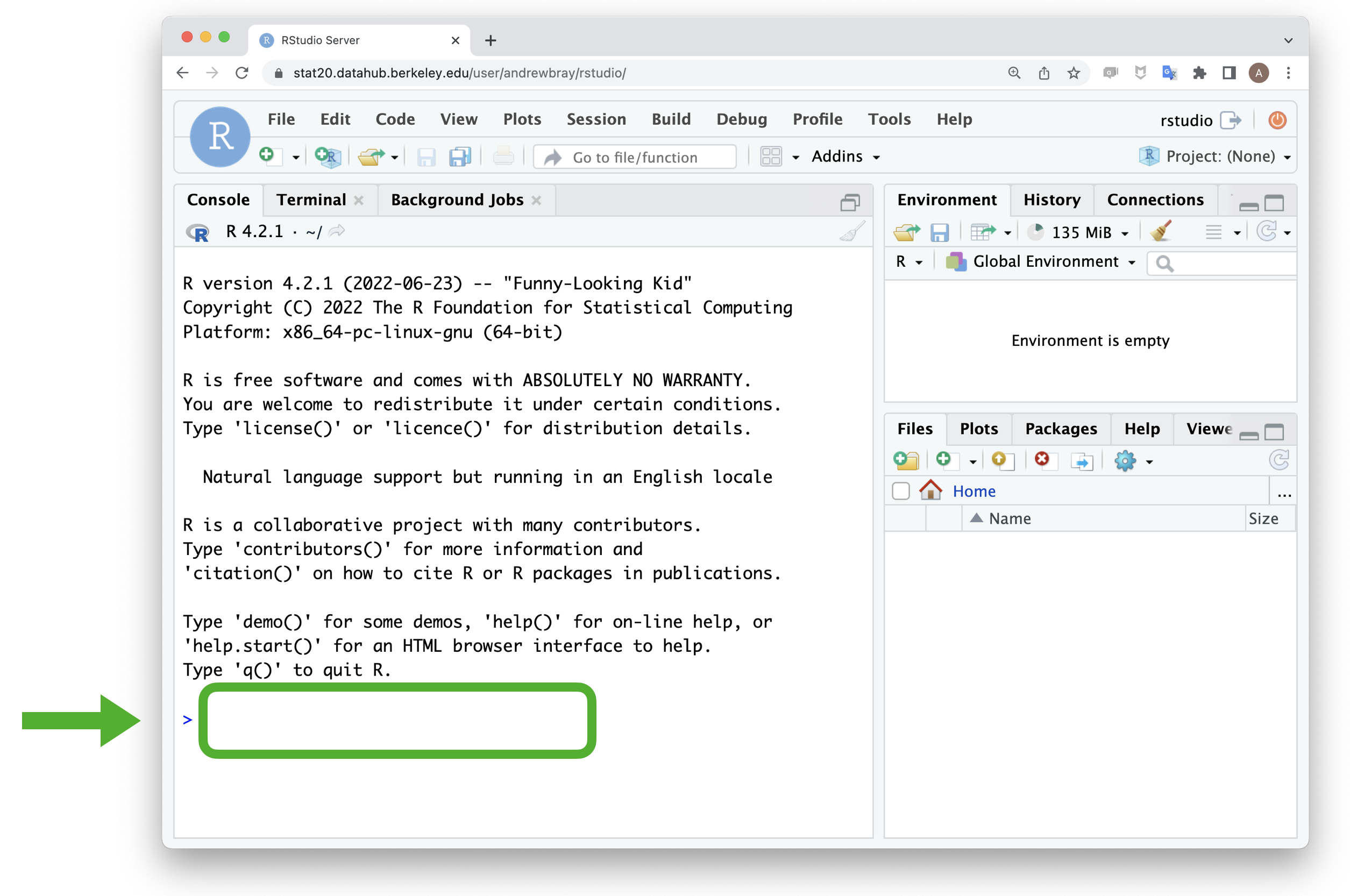
As you read through these notes, keep RStudio open in another window to code along at the console.

R as a Calculator

Although R is capable of running sophisticated statistical models, it’s also more than able to act as a calculator. Type the sum 1 + 2 into the console (the area to the right of the >) and press Enter. What you should see is this:

1 + 2

[1] 3

All of the arithmetic operations work in R.

1 - 2

[1] -1

1 * 2

[1] 2

1 / 2

[1] 0.5

Each of these four lines of code is called a command and the response from R is the output. The [1] at the beginning of the output is there just to indicate that it is the first element of the output. This helps you keep track of things when the output spans many lines.

Although it is easiest to read code when the numbers are separated from the operator by a single space, it’s not necessary. R ignores all spaces when it runs your code, so each of the following also work.

1/2

[1] 0.5

1   /         2

[1] 0.5

You can add exponents by using ^, but don’t forget about the order of operations. If you want an alternative ordering, use parentheses.

2 ^ 3 + 1

[1] 9

2 ^ (3 + 1)

[1] 16

Saving Objects

Whenever you want to save the output of an R command, add an assignment arrow <- (less than, minus) as well as a name, such as “answer” to the left of the command.

answer <- 2 ^ (3 + 1)

When you run this command, there are two things to notice.

1. The word answer appears in the upper right hand corner of RStudio, in the “Environment” tab.
2. No output is returned at the console.

Every time you run a command, you can ask yourself: do I want to just see the output at the console or do I want to save it for later? If the latter, you can always see the contents of what you saved by just typing its name at the console and pressing Enter.

answer

[1] 16

There are a few rules around the names that R will allow for the objects that you’re saving. First, while all letters are fair game, special characters like +, -, /, !, $, are off-limits. Second, names can contain numbers, but not as the first character. That means names like answer, a, a12, my_pony, and FOO will all work. 12a and my_pony! will not.

But just because I’ve told you that those names won’t work doesn’t mean you shouldn’t give it a try…

my_pony! <- 2 ^ (3 + 1)

Error: <text>:1:8: unexpected '!'
1: my_pony!
           ^

This is an example of an error message and, though they can be alarming, they’re also helpful in coaching you how to correct your code. Here, it’s telling you that you had an “unexpected !” and then it points out where in your code that character popped up.

Creating Vectors

While it is helpful to be able to store a single number as an R object, to store data sets we’ll need to store a series of numbers. You can combine multiple values by putting them inside c() separated by commas.

my_fav_numbers <- c(9, 11, 19, 28)
my_fav_numbers

[1]  9 11 19 28

This is object is called a vector.

Vector (in R)

A set of contiguous data values that are of the same type.

As the definition suggests, you can create vectors out of many different types of data. To store words as data, use the following:

my_fav_colors <- c("green", "orange", "purple")
my_fav_colors

[1] "green"  "orange" "purple"

As this example shows, R can store more than just numbers as data. "green", "orange“, and "purple" are each called character strings and when combined together with c() they form a character vector. You can identify a string because it is wrapped in quotation marks and gets highlighted a different color in RStudio.

Vectors are often called atomic vectors because, like atoms, they are the simplest building blocks in the R language. Most of the objects in R are, at the end of the day, constructed from a series of vectors.

Functions

While the vector will serve as our atomic method of storing data in R, how do we perform computations on it? That is the role of functions.

Let’s use a function to find the arithmetic mean of the vector my_fav_numbers.

mean(my_fav_numbers)

[1] 16.75

A function in R operates in a very similar manner to functions that you’re familiar with from mathematics.

Figure 2: A mathematical function as a box with inputs and outputs.

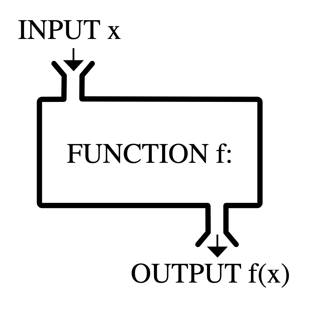
In math, you can think of a function, \(f()\) as a black box that takes the input, \(x\), and transforms it to the output, \(y\). You can think of R functions in a very similar way. For our example above, we have:

• Input: the vector of four numbers that serves as the input to the function, my_fav_numbers.
• Function: the function name, mean, followed by parentheses.
• Output: the number 16.75.

Functions on Vectors

mean() is just one of thousands of different functions that are available in R. Most of them are sensibly named, like the following, which compute square roots and natural logarithms.

By default, log() computes the natural log. To use other bases, see ?log.

sqrt(my_fav_numbers)

[1] 3.000000 3.316625 4.358899 5.291503

log(my_fav_numbers)

[1] 2.197225 2.397895 2.944439 3.332205

Note that with these two functions, the input was a vector of length four and the output is a vector of length four. This is a distinctive aspect of the R language and it is helpful because it allows you to perform many separate operations (taking the square root of four numbers, one by one) with just a single command.

The Taxonomy of Data in R

In the last lecture notes, we introduced the Taxonomy of Data as a broad system to classify the different types of variables on which we can collect data. If you recall, a variable is a characteristic of an object that you can measure and record. When Dr. Gorman walked up to her first penguin (the unit of observation) and measured its bill length, she collected a single observation of the variable bill_length_mm. You could record that in R using,

bill_length_mm <- 50.7

She continued on to measure the next penguin, then the next, then the next… Instead of recording these as separate objects, it is more efficient to store them as a vector.

bill_length_mm <- c(50.7, 48.5, 52.8, 44.5, 42.0, 46.9, 50.2, 37.9)

This example shows that

A vector in R is a natural way to store observations on a variable.

so in the same way that we have asked, “what is the type of that variable?” we can now ask “what is the class of that variable in R?”.

Class (R)

A collection of objects, often vectors, that share similar attributes and behaviors.

While there are many classes in R, you can get a long way only knowing three. The first is represented by our vector my_fav_numbers. Let’s check it’s class using the class() function.

class(my_fav_numbers)

[1] "numeric"

Here we learn that my_fav_numbers is a numeric vector. Numeric vectors, as the name suggests, are composed only of numbers and can include measurements from both discrete and continuous numerical variables.

What about my_fav_colors?

class(my_fav_colors)

[1] "character"

R stores that as a character vector. This is a very flexible class that can be used to store text as data. But what if there are only a few fixed values that a variable can take? In that case, you can do better than a character vector by usinggit a factor. Factor is a very useful class in R because it encodes the notion of levels discussed in the last notes.

To illustrate the difference, let’s make a character vector but then enrich it by turning it into a factor using factor().

char_vec <- c("cat", "cat", "dog")
fac <- factor(char_vec)
char_vec

[1] "cat" "cat" "dog"

fac

[1] cat cat dog
Levels: cat dog

The original character vector stores the same three strings that we used as input. The factor adds some additional information: the possible values that this vector can take.

This is particularly useful when you want to let R know that these levels have a natural ordering. If you have strong opinions about the relative merit of dogs over cats, you could specify that using:

ordered_fac <- factor(char_vec, levels = c("dog", "cat"))
ordered_fac

[1] cat cat dog
Levels: dog cat

This example also demonstrates that you can create a (character) vector inside a function.

While this doesn’t change the way the levels are ordered in the vector itself, it will effect the way they behave when we use them to create plots, as we’ll do in the next set of notes.

These three vector classes do a good job of putting into flesh and bone (or at least silicon) the abstract types captured in the Taxonomy of Data.

Figure 3: The Taxonomy of Data with equivalent classes in R.

Data Frames in R

While vectors in R do a great job of capturing the notion of a variable, we will need more than that if we’re going to represent something like a data frame. Conveniently enough, R has a structure well-suited to this task called…(drumroll…)

Dataframe (R)

A two dimensional data structure used to store vectors of the same length. A direct analog of the data frame defined previously⁵.

Let’s use R to recreate the penguins data frame collected by Dr. Gorman.

bill_length_mm	bill_depth_mm	species
43.5	18.1	Chinstrap
48.1	15.1	Gentoo
49.0	19.5	Chinstrap
45.4	18.7	Chinstrap
34.6	21.1	Adelie
49.8	17.3	Chinstrap
40.9	18.9	Adelie
45.3	13.7	Gentoo

Creating a data frame

In the data frame above, there are three variables; the first two numeric continuous, the last one categorical nominal. Since R stores variables as vectors, we’ll need to create three vectors.

bill_length_mm <- c(50.7, 48.5, 52.8, 44.5, 42.0, 46.9, 50.2, 37.9)
bill_depth_mm <- c(19.7, 15.0, 20.0, 15.7, 20.2, 16.6, 18.7, 18.6)
species <- factor(c("Chinstrap", "Gentoo", "Chinstrap", "Gentoo", "Adelie", 
             "Chinstrap", "Chinstrap", "Adelie"))

While bill_length_mm and bill_depth_mm are both being stored as numeric vectors, species was first collected into a character vector, then passed directly to the factor() function. This is an example of nesting one function inside of another and it combined two lines of code into one.

With the three vectors stored in the Environment, all you need to do is staple them together with data.frame().

penguins_df <- data.frame(bill_length_mm, bill_depth_mm, species)
penguins_df

  bill_length_mm bill_depth_mm   species
1           50.7          19.7 Chinstrap
2           48.5          15.0    Gentoo
3           52.8          20.0 Chinstrap
4           44.5          15.7    Gentoo
5           42.0          20.2    Adelie
6           46.9          16.6 Chinstrap
7           50.2          18.7 Chinstrap
8           37.9          18.6    Adelie

Summary

This was our first introduction to R, a supercharged calculator for storing and computing on data. We learned how to do basic arithmetic, construct and save a vector, call functions, query the class of an object, and construct a data frame. This forms the foundation of our use of R. If that foundation feels shakey, don’t fret. We’ll get plenty of practice in class.

Figure 4: The arc of learning R⁶.

Exercises

Ex: R as a Calculator

Meet Leia, a fictitious undergrad student taking Stat 20. Leia loves to drink coffee in the morning, and she brews her own coffee at home. She even has a monthly budget of $20 to cover this type of expense. As you know, we can use R to create an object or variable coffee for Leia’s budget:

coffee <- 20

Alternatively, you can also use the equals sign = as an assignment operator:

coffee = 20

Your Turn: Leia’s Expenses

Consider the bills of Leia’s fixed monthly expenses:

• phone $80
• transportation $20
• groceries $600
• rent $1800

1. Make more assignments to create variables phone, transportation, groceries, and rent with their corresponding amounts.

Solution:

phone <- 80
transportation <- 20
groceries <- 600
rent <- 1800

/

2. Now that you have all the variables, create a total object with the sum of her fixed monthly expenses.

Solution:

total <- phone + transportation + groceries + rent
total

/

3. Assuming that Leia has the same expenses every month, how much would she spend during a school “semester”? (assume the semester involves five months).

Solution:

total * 5

/

4. Maintaining the same assumption about the monthly expenses, how much would Leia spend during a school “year”? (assume the academic year is 10 months).

Solution:

total * 10

/

Ex: Taxonomy of Data and R Vectors

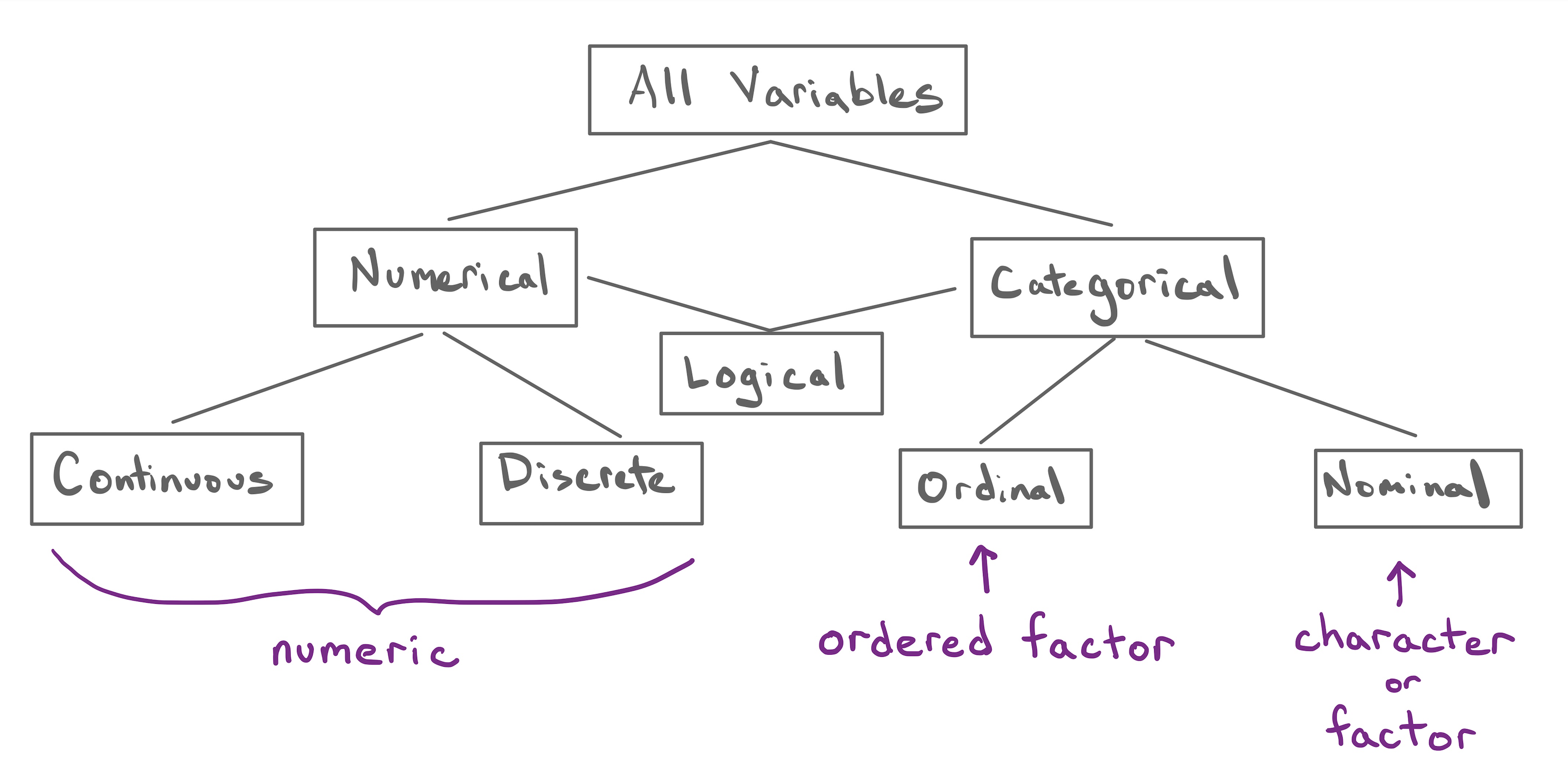
From the taxonomy of data, you know that we have 4 flavors of variables, and their corresponding classes in R (shown below inside parenthesis) illustrated in the following examples:

# continuous (numeric)
x1 <- c(1.2, 3.3, -0.5)

# discrete (numeric)
x2 <- c(2, 4, 6)

# ordinal (ordered factor)
x3 <- factor(c("sm", "md", "lg", "sm"), levels = c("sm", "md", "lg"))

# nominal (character or factor)
x4 <- c("strawberry", "lemon", "vanilla")
x4bis <- factor(c("strawberry", "lemon", "vanilla"))

Your Turn: Terrestrial Planets

Consider the following data set—shown in the table below—containing variables of so-called Terrestrial planets. These planets include Mercury, Venus, Earth, and Mars. They are called like this because they are “Earth-like” planets: relatively small in size and in mass, with a solid rocky surface, and metals deep in its interior.

name	gravity	moons
Mercury	3.7	0
Venus	8.9	0
Earth	9.8	1
Mars	3.7	2

/

1. Consider the column name in the provided table of terrestrial planets. Use the c() function to create a character vector name containing the names of the Terrestrial planets.

Solution:

name = c("Mercury", "Venus", "Earth", "Mars")

/

2. Consider the column gravity in the provided table of terrestrial planets. Use the combine function c() to make a numeric vector gravity for the Terrestrial planets.

Solution

gravity = c(3.7, 8.9, 9.8, 3.7)

/

3. Consider the column moons in the provided table of terrestrial planets. Use the combine function c() to make an ordinal factor moons.

Solution

moons = factor(c(0, 0, 1, 2), ordered = TRUE)

/

Ex: Data Frames in R

Consider again the data set of Terrestrial planets—shown in the table below.

name	gravity	moons
Mercury	3.7	0
Venus	8.9	0
Earth	9.8	1
Mars	3.7	2

/

Use the vectors that you defined in the previous section in order to create a data frame planets:

Solution

planets = data.frame(
  "name" = name,
  "gravity" = gravity,
  "moons" = moons,
  "haswater" = haswater
)

/

Ex: Challenge

Let’s apply everything that you’ve learned so far in order to create a data frame students containing the following data, and the provided specifications listed below:

name	height	year	resident
Leia	160	sophomore	TRUE
Luke	170	freshman	FALSE
Han	182	senior	TRUE
Lando	178	junior	FALSE

/

• name: nominal variable (character)
• height continuous variable (numeric)
• year: ordinal variable (ordered factor)
• resident: nominal variable (logical)

Solution

students = data.frame(
  "name" = c("Leia", "Luke", "Han", "Lando"),
  "height" = c(160, 170, 182, 178),
  "year" = factor(x = c("sophomore", "freshman", "senior", "junior"),
                  levels = c("freshman", "sophomore", "junior", "senior")),
  "resident" = c(TRUE, FALSE, TRUE, FALSE)
)

References and further reading

• Hands on Programming with R by Garret Grolemund. A friendly introduction to the R language with fun examples.

• The official (somewhat dense) documentation fo the R language. https://cran.r-project.org/doc/manuals/r-release/R-lang.html

• R for Data Science by Hadley Wickham and Garrett Grolemund. A comprehensive but approachable guide to doing data science with R. A good reference once you’re deeper into this course..

Footnotes

1. The googlesheets4 package, which reads spreadsheet data into R was authored by Jenny Bryan, a developer at Posit: :https://googlesheets4.tidyverse.org/.

2. The statistics office of the province of British Columbia maintains a public R package with all of their data: https://bcgov.github.io/bcdata/

3. Dr. Christopher Paciorek in the Department of Statistics at UC Berkeley maintains a package to fit a very broad class of statistical models called Bayesian Models: https://r-nimble.org/.

4. Simon Couch wrote the stacks package for model ensembling while an undergraduate https://stacks.tidymodels.org/index.html.

5. R is an unusual language in that the data frame has been for decades a core structure of the language. The analogous structure in Python is the data frame found in the Pandas library.

6. R monster artwork by @allison_horst.