Data Wrangling

STAT 20: Introduction to Probability and Statistics

Warmup Questions

This is a code heavy day, so it can be helpful to write up the names of the key dplyr verbs - mutate, arrange, select, filter, summarize, group_by - on side boards at the beginning when write short definitions as they come up. They can serve as references for the rest of the class period.

It can also be helpful to have RStudio open so that you can copy and paste from these cells into RStudio and run them.

What will this line of code return?

c("smile", "frown", "smile") == "frown"

FALSE TRUE FALSE

Rewrite this nested function call using pipes

exp(mean(c(1, 2, 3, NA), na.rm = TRUE))

c(1, 2, 3, NA) |> mean(na.rm = TRUE) |> exp()

Or even:

1 |> c(2, 3, NA) |> sum() |> exp()!

Filtering

flights |>
  filter(dep_time >= 22,
         carrier %in% c("UA", "AA"),
         dep_delay <= 0)

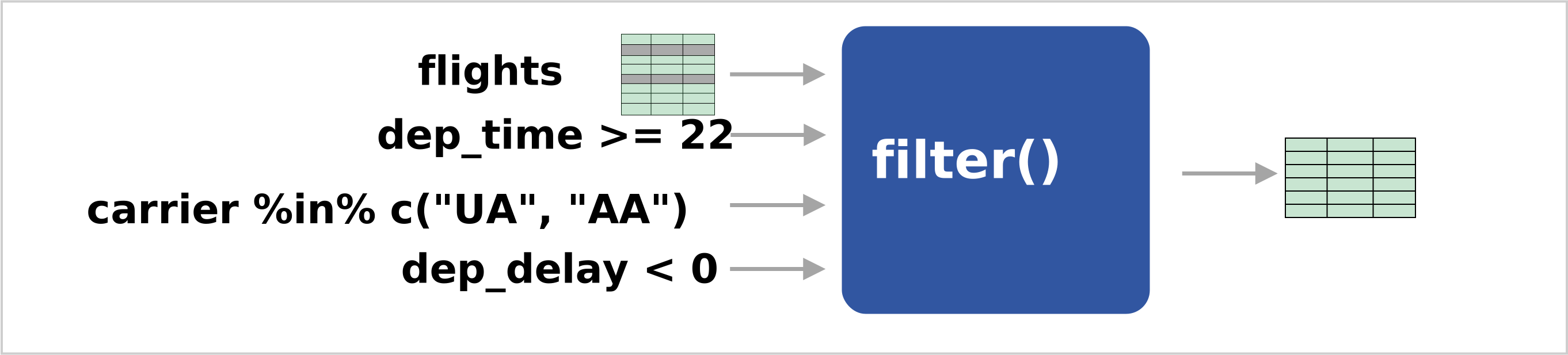
Which observations will be included in the data frame produced by this code? Or equivalently, which observations will not be included?

Just write a few English sentences describing what flights will remain in the new dataframe…

Only those flights who fit all of the following criteria will appear in the resulting data frame:

1. Departed at 10pm or later.
2. Were operated by United Airlines or American Airlines.
3. Departed on time or early.

Which data frame will have fewer rows?

# A
filter(flights, origin == "OAK")

# B
flights |>
  mutate(from_oakland = (origin == "OAK")) |>
  filter(from_oakland)

Neither, they’ll have the same number of rows. The second approach just creates a new column along the way.

Build a pipeline

Write a code pipeline that extracts, from the penguins dataframe, only Adelie penguins with bill lengths between 40 and 45mm.

Solution 1:

penguins |>
  filter(species == "Adelie" & bill_length_mm >= 40 & bill_length_mm <= 45)

Solution 2:

penguins |>
  filter(species == "Adelie", bill_length_mm >= 40, bill_length_mm <= 45)

What does this line of code compute?

penguins |>
  mutate(chonky = body_mass_g > 3500) |>
  summarize(mean(chonky))

Answer in an English sentence. Nevermind what actual number it will produce, just explain what that number will mean.

The proportion of penguins that weigh more than 3500 grams.

Building Data Pipelines

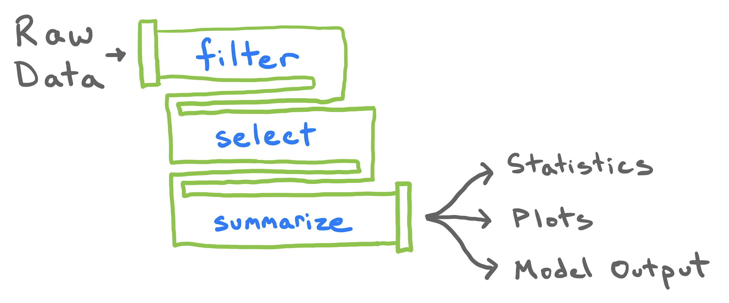
Building Data Pipelines

Consider the subset of flights here:

filter(flights,
       dep_time >= 22,
       carrier %in% c("UA", "AA"),
       dep_delay <= 0)

How do we extract the average departure delay for each airline in this subset of flights?

Let’s look at three different ways to answer this question

This set of slides walks through the three different approaches to stringing together functions in R, identifies the pros and cons of each, and encourages students to use the pipe.

Nesting

filter(flights,
       dep_time >= 22,
       carrier %in% c("UA", "AA"),
       dep_delay <= 0)

Nesting

group_by(filter(flights,
       dep_time >= 22,
       carrier %in% c("UA", "AA"),
       dep_delay <= 0),
       carrier)

Nesting

summarize(group_by(filter(flights,
       dep_time >= 22,
       carrier %in% c("UA", "AA"),
       dep_delay <= 0),
       carrier),
       avg_dep_delay = mean(dep_delay))

# A tibble: 2 × 2
  carrier avg_dep_delay
  <chr>           <dbl>
1 AA              -6.43
2 UA              -5.88

Nesting

summarize(group_by(filter(flights,
       dep_time >= 22,
       carrier %in% c("UA", "AA"),
       dep_delay <= 0),
       carrier),
       avg_dep_delay = mean(dep_delay))

Nesting

summarize(group_by(filter(flights,
       dep_time >= 22,
       carrier %in% c("UA", "AA"),
       dep_delay <= 0),
       carrier),
       avg_dep_delay = mean(dep_delay))

Cons

• Must be read from inside out
• Hard to keep track of arguments

Pros

• All in one line of code
• Only refer to one data frame

Make intermediate variables

df1 <- filter(
       flights,
       dep_time >= 22,
       carrier %in% c("UA", "AA"),
       dep_delay <= 0)
df2 <- group_by(df1, carrier)
summarize(df2,
          avg_dep_delay = mean(dep_delay))

Cons

• Have to repeat data frame names
• Creates unnecessary objects

Pros

• Stores intermediate objects
• Can be read top to bottom

Quick refresh: the pipe operator

sqrt(16)

[1] 4

The pipe operator |> takes whatever is on the left side of the pipe and inserts it as the first argument of the function on the right side.

So the above can be rewritten as…

16 |> sqrt()

[1] 4

Pipelines using the pipe operator |>

flights |>
  filter(dep_time >= 22,
         carrier %in% c("UA", "AA"),
         dep_delay <= 0) |>
  group_by(carrier) |>
  summarize(avg_dep_delay = mean(dep_delay))

Compare this to the nested approach:

summarize(group_by(filter(flights,
       dep_time >= 22,
       carrier %in% c("UA", "AA"),
       dep_delay <= 0),
       carrier),
       avg_dep_delay = mean(dep_delay))

Pipelines using the pipe operator |>

flights |>
  filter(dep_time >= 22,
         carrier %in% c("UA", "AA"),
         dep_delay <= 0) |>
  group_by(carrier) |>
  summarize(avg_dep_delay = mean(dep_delay))

Notice how it the code now more naturally follows the diagram (piped-in arguments are annotated with |>)

Pipelines using the pipe operator |>

flights |>
  filter(dep_time >= 22,
         carrier %in% c("UA", "AA"),
         dep_delay <= 0) |>
  group_by(carrier) |>
  summarize(avg_dep_delay = mean(dep_delay))

Cons

• Not too many!

Pros

• Can be read like an english paragraph
• Only type the data once
• No leftovers objects

Breaking the pipe

It’s good practice to understand the output of each line of code by breaking the pipe. That is, cut off some pipeline steps and see if the output-so-far looks right.

flights |>
  filter(dep_time >= 22,
         carrier %in% c("UA", "AA"),
         dep_delay <= 0) |>
  group_by(carrier) |>
  summarize(avg_dep_delay = mean(dep_delay))

carrier	avg_dep_delay
AA	-6.433027
UA	-5.876621

First step only

flights |>
  filter(dep_time >= 22,
         carrier %in% c("UA", "AA"),
         dep_delay <= 0)

carrier	dep_time	dep_delay
AA	555	-5
UA	1039	-12
UA	1052	-8
AA	1853	-6
AA	848	-12

First two steps

flights |>
  filter(dep_time >= 22,
         carrier %in% c("UA", "AA"),
         dep_delay <= 0) |>
  group_by(carrier)

carrier	dep_time	dep_delay
AA	555	-5
UA	1039	-12
UA	1052	-8
AA	1853	-6
AA	848	-12

Full pipeline

flights |>
  filter(dep_time >= 22,
         carrier %in% c("UA", "AA"),
         dep_delay <= 0) |>
  group_by(carrier) |>
  summarize(avg_dep_delay = mean(dep_delay))

carrier	avg_dep_delay
AA	-6.433027
UA	-5.876621

Worksheet: Conditioning

20:00

Break

05:00

Lab Part I: Flights

25:00